

Price Action And Python Forex
By Milind Paradkar
This blog highlights six technical indicators and how they can be coded using Python. These technical indicators are popularly used in the markets to study the toll movement.
- Commodity Channel Index
- Ease of Movement
- Moving Average
- Charge per unit of Change
- Bollinger Bands
- Force Alphabetize
A brief introduction to Technical Indicators
A Technical Indicator is essentially a mathematical representation based on data sets such as price (high, depression, open, close, etc.) or volume of security to forecast price trends.
In that location are several kinds of technical indicators that are used to analyse and detect the direction of movement of the price (for momentum trading, mean reversion trading etc). Traders use them to study the short-term toll movement since they practise non bear witness very useful for long-term investors. They are employed primarily to predict futurity price levels.
Technical Indicators do not follow a general pattern, meaning, they behave differently with every security. What can be a skilful indicator for a detail security, might non hold the example for the other. Thus, using a technical indicator requires jurisprudence coupled with good feel.
As these analyses tin be washed in Python, a snippet of code is as well inserted along with the clarification of the indicators. Sample charts with examples are as well appended for clarity.
Commodity Channel Index
The article channel alphabetize (CCI) is an oscillator that was originally introduced past Donald Lambert in 1980. CCI can be used to identify cyclical turns across nugget classes, be it bolt, indices, stocks, or ETFs. Traders also use CCI to identify overbought/oversold levels for securities.
Estimation
The CCI looks at the relationship between price and a moving average. Steps involved in the interpretation of CCI include:
- Compute the typical price for security. The typical price is obtained by averaging the high, low and close cost for the day.
- Calculate the simple moving average of the typical prices for the chosen number of days.
- Compute the mean deviation of typical prices for the same menstruation every bit that used for the moving boilerplate.
Formula for the Commodity Aqueduct Index
The formula for CCI is given by:
CCI = (Typical price – MA of Typical toll) / (0.015 * mean deviation of Typical price) 0.015 is Lambert's constant.
Analysis
CCI can be used to make up one's mind overbought and oversold levels.
- Readings above +100 tin imply an overbought condition
- Readings below −100 can imply an oversold condition.
Notwithstanding, 1 should be conscientious considering security can proceed moving higher later the CCI indicator becomes overbought. Likewise, securities can go on moving lower later on the indicator becomes oversold.
Whenever the security is in overbought/oversold levels as indicated by the CCI, there is a skilful chance that the price will come across corrections. Hence a trader can apply such overbought/oversold levels to enter in brusk/long positions.
Traders can too wait for divergence signals to take suitable positions using CCI. A bullish divergence occurs when the underlying security makes a lower depression, and the CCI forms a college depression, which shows less downside momentum.
Similarly, a bearish divergence is formed when the security records a higher high and the CCI forms a lower high, which shows less upside momentum.
Python lawmaking for computing the Commodity Aqueduct Index
In the code below, we use the rolling(), mean(), and mad() functions to compute the Commodity Channel Index. The rolling and hateful function takes a fourth dimension series or a data frame along with the number of periods and computes the rolling mean.
The mad() office computes the mean deviation based on the price provided.
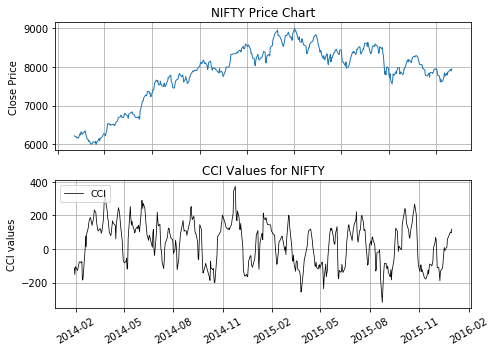
Nosotros have too plotted the NIFTY Price series and the Commodity Channel Index (CCI) values. We first create an empty figure using the plt.effigy function and then create two subplots.
The commencement subplot charts the NIFTY cost series, while the second subplot charts the CCI values.
Go to the Peak
Ease of Move
Ease of Movement (EVM) is a volume-based oscillator which was developed by Richard Arms. EVM indicates the ease with which the prices rise or fall taking into business relationship the volume of the security.
For example, a price rise on a low book means prices advanced with relative ease, and there was little selling pressure level. Positive EVM values imply that the market place is moving higher with ease, while negative values betoken an easy decline.
Interpretation
To calculate the EMV we first calculate the distance moved. It is given by:
Distance moved = ((Current High + Current Low)/2 - (Prior Loftier + Prior Low)/2)
We then compute the Box ratio which uses the volume and the high-low range:
Box ratio = (Book / 100,000,000) / (Current High – Electric current Low) EMV = Altitude moved / Box ratio
To compute the n-period EMV we have the northward-period simple moving boilerplate of the 1-period EMV.
Analysis
Ease of Movement (EMV) can exist used to confirm a bullish or a bearish trend. A sustained positive Ease of Movement together with a rising marketplace confirms a bullish trend, while a negative Ease of Movement values with falling prices confirms a bearish tendency. Apart from using equally a standalone indicator, Ease of Movement (EMV) is also used with other indicators in nautical chart assay.
Python code for computing the Ease of Movement (EMV)
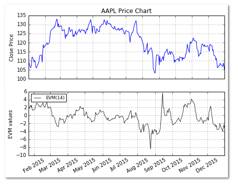
Example code: fourteen-mean solar day Ease of Movement (EMV) for AAPL.
In the code below we apply the Series, rollingmean, shift, and the join functions to compute the Ease of Movement (EMV) indicator. The Serial role is used to form a series which is a 1-dimensional array-like object containing an array of data.
The rollingmean function takes a time series or a data frame along with the number of periods and computes the mean. The shift function is used to fetch the previous day's high and low price. The join function joins a given series with a specified serial/dataframe.
We have also plotted the AAPL Price series and the Ease of Move (EVM) values below the price chart. Nosotros first create an empty effigy using the plt.effigy function and and then create two subplots. The first subplot charts the AAPL cost series, while the second subplot charts the EVM values.
Go to the Pinnacle
Moving Average
The moving average is i of the most widely used technical indicators. Information technology is used along with other technical indicators or information technology can form the building block for the computation of other technical indicators.
A "moving average" is the average of the asset prices over the "10" number of days/weeks. The term "moving" is used considering the group of data moves frontward with each new trading 24-hour interval. For each new solar day, nosotros include the price of that twenty-four hours and exclude the price of the commencement day in the data sequence.
The most commonly used moving averages are the 5-24-hour interval, 10-twenty-four hour period, 20-24-hour interval, 50-day, and the 200-day moving averages.
Estimation
There are different types of moving averages used for analysis, a elementary moving average (SMA), weighted moving boilerplate (WMA), and the exponential Moving boilerplate (EMA).
To compute a twenty-day SMA, we accept the sum of prices over 20 days and separate information technology by 20. To arrive at the next data point for the 20-twenty-four hours SMA, we include the price of the next trading day while excluding the toll of the starting time trading 24-hour interval. This way the group of data moves forward.
The SMA assigns equal weights to each cost betoken in the group. When we compute a twenty-day WMA, we assign varying weights to each toll points. The latest toll, i.e. the 20th-twenty-four hours price gets the highest weightage, while the first price gets the lowest weightage. This sum is so divided past the sum of the weights used.
To compute the 20-solar day EMA, nosotros commencement compute the very start EMA value using a uncomplicated moving average. Then we calculate the multiplier, and thereafter to compute the second EMA value we utilize the multiplier and the previous day EMA. This formula is used to compute the subsequent EMA values.
SMA: xx catamenia sum / twenty Multiplier: (2 / (Time periods + ane)) = (2 / (xx + ane)) = ix.52% EMA: {Close price - EMA(previous day)} x multiplier + EMA(previous day). Analysis
The moving average tells whether a trend has begun, concluded or reversed. The averaging of the prices produces a smoother line which makes it easier to identify the underlying trend. However, the moving boilerplate lags the market activity.
A shorter moving average is more than sensitive than a longer moving boilerplate. However, it is prone to generate false trading signals.
Using a single Moving Boilerplate – A single moving average tin exist used to generate trade signals. When the closing price moves above the moving average, a buy signal is generated and vice versa. When using a single moving average 1 should select the averaging period in such a way that it is sensitive in generating trading signals and at the same time insensitive in giving out simulated signals.
Using two Moving Averages – Using a unmarried moving boilerplate can exist disadvantageous. Hence many traders use two moving averages to generate signals. In this case, a buy signal is generated when the shorter average crosses higher up the longer average. Similarly, a sell is generated when the shorter crosses below the longer average. Using two moving averages reduces the fake signals which are more than probable when using a unmarried moving average.
Traders also utilize three moving averages, like the v, 10, and xx-day moving average system widely used in the commodity markets.
Python code for computing Moving Averages for Not bad
In the code beneath nosotros utilize the Series, rolling hateful, and the join functions to create the SMA and the EWMA functions. The Series function is used to form a serial which is a one-dimensional assortment-like object containing an array of data.
The rolling_mean function takes a time series or a data frame along with the number of periods and computes the hateful. The join office joins a given series with a specified series/dataframe.
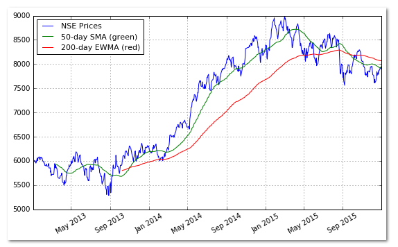
Nosotros accept also plotted the Swell cost serial, 50-twenty-four hours SMA, and the 200-day EWMA.
Get to the Tiptop
Rate of Change
The Rate of Change (ROC) is a technical indicator that measures the percent alter between the most recent cost and the price "n" day'south ago. The indicator fluctuates effectually the nada line.
If the ROC is ascension, it gives a bullish signal, while a falling ROC gives a bearish bespeak. One can compute ROC based on dissimilar periods in order to guess the curt-term momentum or long-term momentum.
Estimation
ROC = [(Close price today - Shut cost "n" solar day'south agone) / Close price "n" twenty-four hour period's ago))]
Python code for computing Charge per unit of Change (ROC)
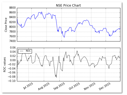
Example code: 5-day Rate of Modify (ROC) for NIFTY.
In the code below we use the Series, diff, shift, and the join functions to compute the Rate of Change (ROC). The Series function is used to form a series which is a one-dimensional array-like object containing an array of data.
The unequal office computes the difference in prices between the current day's toll and the cost "n" day'southward ago. The shift role is used to fetch the previous "northward" day'southward price. The join function joins a given serial with a specified series/dataframe.
We have as well plotted the Cracking Price series and the Charge per unit of Change (ROC) values below the price chart. We offset create an empty figure using the plt.figure function and then create ii subplots.
The first subplot charts the NIFTY price series, while the 2d subplot charts the ROC values.
Get to the Top
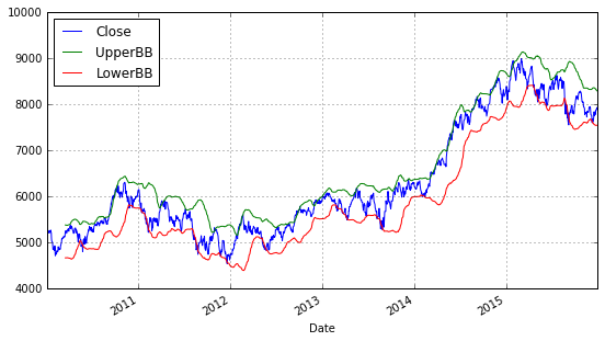
Bollinger Bands
The concept of Bollinger bands was developed past John Bollinger. These bands comprise of an upper Bollinger band and a lower Bollinger ring and are placed ii standard deviations above and below a moving average.
Bollinger bands expand and contract based on the volatility. During a catamenia of ascent volatility, the bands widen, and they contract every bit the volatility decreases. Prices are considered to exist relatively high when they motion above the upper band and relatively low when they go below the lower band.
Estimation
To create the bands, we first compute the SMA and then apply this to compute the bands values.
Middle Ring = twenty-day uncomplicated moving boilerplate (SMA) Upper Band = 20-day SMA + (2 ten 20-twenty-four hour period standard departure of cost) Lower Ring = twenty-24-hour interval SMA - (two x 20-day standard deviation of price)
Analysis
To utilise Bollinger bands for generating signals, a uncomplicated approach would be to utilise the upper and the lower bands every bit the cost targets. If the price bounces off the lower band and crosses the moving average line, the upper band becomes the upper price target.
In the case of a crossing of the toll beneath the moving average line, the lower ring becomes the downside target price.
Python code for computing Bollinger Bands for Smashing
In the code beneath we rolling office to create the Bollinger band function. The hateful and the standard difference methods are used to compute these respective metrics using the close price.
One time we have computed the hateful and the standard deviation, we compute the upper Bollinger band and the lower Bollinger band. The Bollinger ring part is called on the Slap-up price data using the 50-24-hour interval moving average window.
Go to the Meridian
Force Index
The strength index was created by Alexander Elder. The force index takes into business relationship the direction of the stock price, the extent of the stock price movement, and the volume. Using these three elements it forms an oscillator that measures the buying and the selling pressure.
Each of these three factors plays an important role in the determination of the force index. For case, a big advance in prices, which is given by the extent of the price motility, shows a strong ownership pressure. A large decline in heavy volume indicates a strong selling pressure.
Interpretation
Example: Computing Strength index(1) and Forcefulness index(fifteen) catamenia.
The Strength index(1) = {Close (current period) - Close (prior catamenia)} x Current period Volume The Forcefulness Index for the 15-day catamenia is an exponential moving boilerplate of the 1-period Force Index.
Analysis
The Force Alphabetize can exist used to decide or confirm the tendency, identify corrections and foreshadow reversals with divergences. A shorter force index is used to determine the curt-term tendency, while a longer strength index, for example, a 100-day forcefulness alphabetize tin can be used to decide the long-term trend in prices.
A force index can also be used to identify corrections in a given trend. To do and so, it can be used in conjunction with a trend following indicator. For instance, i can use a 22-day EMA for tendency and a 2-solar day force index to place corrections in the trend.
Python code for computing the Force Index for Apple tree Inc. (AAPL) Stock
In the code beneath we utilize the Series, diff, and the join functions to compute the Force Index. The Series function is used to form a series which is a one-dimensional assortment-like object containing an array of data.
The unequal function computes the difference betwixt the electric current data point and the data indicate "n" periods/days apart. The join part joins a given series with a specified serial/dataframe.
Go to the Top
Learn how to use Seaborn Python package to create Heatmaps for data visualisation which can exist used for various purposes, including by traders for tracking markets.
If you are seeking more than information on Python libraries for Algo Trading, check out our this weblog.
Learning and implementing different trading strategies in your trading is possible. Quantra'south bundle of courses provide knowledge of algorithmic trading for everyone. They're perfect for traders and quants who want to learn and use Python in trading. Enroll now!
Update: Nosotros have noticed that some users are facing challenges while downloading the market information from Yahoo and Google Finance platforms. In example you are looking for an alternative source for market information, you tin employ Quandl for the same. Disclaimer: All investments and trading in the stock marketplace involve take chances. Whatsoever decisions to place trades in the financial markets, including trading in stock or options or other financial instruments is a personal determination that should only be made after thorough research, including a personal risk and financial cess and the date of professional assistance to the extent you believe necessary. The trading strategies or related information mentioned in this article is for informational purposes only.
Files in the download
- Commodity Channel Index (CCI) - Python code
- Ease of Movement (EVM) - Python code
- Moving Boilerplate (MA) - Python code
- Rate of Modify (ROC) - Python code
- Bollinger Bands - Python code
- Force Index - Python lawmaking
Login to Download

Source: https://blog.quantinsti.com/build-technical-indicators-in-python/
Posted by: conerlydeggence.blogspot.com
0 Response to "Price Action And Python Forex"
Post a Comment